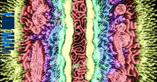
Complex behaviours can arise from simple rules, from cellular automatons to n-body systems and physarum slime mold-inspired simulations - all of these can be used to create fascinating art or simply contemplate the beauty of dynamical systems and chaos. These types of simulations make us ponder that our world perhaps also emerges from very simple rules - indeed in physics we now believe the observable world is the result of the intricate vibrations and interactions of some fairly small number of quantum fields, plus gravity.
One of the types of systems I often come back to is the n-body gravitational simulation. In this type of program, we simulate many (hundreds, thousands, millions?) particles that are able to attract each other through the force of gravity. This type of simulation is often employed in astrophysics and cosmology to create simulations of extremely dense clouds of particles, such as galaxies, resulting in some beautiful renders that also reveal things about how the universe works - for example simulations can model the effects of dark matter on galaxy formation and rotation.
But other than being useful for science stuff, this type of system is great for creating art. Mid-way through working on this experiment I discovered a toy called Particle Life, which does just that, but in a more creative, performable way, and we’ll come back to that later in the article as I took some ideas from it.
I’d like to invite you to take a trip with me down this rabbit hole, and possibly quite long article.
Gravitational N-Body Systems
For this project I used Processing, although I also did a stint in P5.js. I chose Processing in the end because it let me use multi-threading to speed up the calculations. I won’t go extremely deep into the code implementation (it’s not pretty!), and in fact I’ll provide code examples in a more general format as P5 can be quite verbose in its use of things like vectors, but I will try to give an idea of how the basic gravitational n-body problem can be solved and rigged up for “performance”.
Here are the basics of how it works:
There are “Particles”, which have:
P - a position vector
V - a velocity vector
The main loop of the program visits every particle in turn, and for each one then also iterates over all particles. For each one of these pairs we compute a gravitational attraction. For the pair of particles P1, P2 we have:
float distance = dist(P1,P2) //euclidean distance between the particles
vec2 direction = normalize(P2 - P1) //normalized direction from P1 towards P2
vec2 F = direction * (1.0 /(distance*distance))
The variable F is what we care about! It’s also the acceleration caused by P2 on P1. If we want to have different masses, you can also multiply the force by m1 + m2, the masses of the particles (the acceleration would then be based on the mass of the other particle), but my system doesn’t care about masses so we can treat them as 1.0. Because direction is P2 - P1, the direction is from P1 towards P2. The amount of force is 1 over the distance squared, which ideally is also scaled by a constant G (the gravitational constant, which just scales how strong this gravity is).
Once we’ve obtained F by accumulating this for every particle, we can enter the main update of the particle we care about:
V = V + F
P = P + V
This is called Euler integration, and it’s not very good but it does the job to start with. Basically the total acceleration is added to the velocity, and then the velocity is added to the position. Once we’ve done this update for all the particles, we’ll see them whizzing around, being swirled chaotically throughout the world by the gravitational forces of all the other bodies. At this point you can also choose to apply a “delta time” to be able to scale the temporal step we take each time, but let’s assume it’s 1 so we don’t need to do anything.
This approach has a few problems that are worth tackling before trying any more things.
Singularity
Distance Scaling
Accuracy
Performance
Let’s look at them in turn.
Singularity
The equations above have a problem. When the distance between the particles is 0, the force formula divides by 0. Uh oh! Division by 0 is bad enough, but also as the distance gets closer to 0, the forces created tend towards infinity. This is actually related to the concept of a black hole in physics, and it’s something we don’t want in our program. We can tackle this in a few ways:
We can clamp the “potential”, i.e. the force strength calculation to have a minimum distance. This discontinuity can cause some odd unphysical behaviours but I prefer it.
We can use a “Plummer potential” which I read about in an astrophysics book. It replaces the inverse square law formula with one including a square root, but I found this not much better than the clamping method and also a lot more expensive.
We can make the particles collide so they don’t go “inside” each other, and can never go close enough (this is what happens in real life).
I ended up using a simple clamping system in mine. In fact the clamping distance is a parameter I can set and results in quite different visuals. Not everything has to be realistic when we care about art!
Distance Scaling
Depending on what you want to see and how your coordinate system is scaled, you might want to apply a scaling factor to distance. The inverse square has an extremely sharp curve and if the average distance between your particles is on the order of 100s of units/meters, the force will barely show up for particles on different parts of the screen.
Accuracy
The Euler integration above is ok but has a huge problem: it doesn’t conserve energy! This means that the particles can gain velocity from random errors in the integration, resulting in unphysical movements and jittery exploding glitchy orbits. This tends to be extra-bad in situations with lots of forces and no drag/damping. I chose to use something called Verlet Integration, which is much better and is commonly used in games. It isn’t much more complicated but it is a bit slower to compute.
Performance
By far the biggest problem should be evident from how the algorithm works. Visiting every single particle for every single particle is agonizingly slow. It’s an N^2 algorithm, i.e. one of the worst types that will quickly bring your computer to its knees for more than a few hundred particles.
We have a few options here, and a good one is the Quadtree, although the algorithm best suited to this problem is an extension of it called the Barnes-Hut algorithm, which is deceptively simple despite coming from the field of astrophysics.
In a quadtree, we start with a large square (or box). Then we try to add a particle to it. The box has a maximum number of particles that it can contain, and if we exceed this limit, we immediately break up the box into 4 smaller boxes, equally dividing it. Then, we see which of the boxes the particle should be in, and we try to add it there, taking care to first shuffle down the points already existing in the box to their respective new sub-boxes. We do this recursively until we find a box that contains the point and we add it there. Here’s a visualisation of the quadtree squares in my magnet sim (explained later in the article) - notice how emptier areas have sparser subdivision.
To summarise, the boxes are represented by nodes in a tree, and each node can have 4 child nodes, and each node can store up to a maximum of points (1 is a good bet but higher is fine too, and this can be tuned).
Now we can do something magical with this quadtree - use a recursive algorithm to find points nearby to any given point, without searching all the points! This is simple:
Take point A
Create a box around point A, representing the range we are searching in.
Now we will check every quadtree node/box that our query box overlaps.
If it overlaps, we see if it has any points, and then check to see if they’re in the range.
If the box actually has no points but has been split, we go to its children and make the same checks, and we proceed recursively this way until we’ve checked all the boxes we need, but none that are out of range (which eliminates the need to check very many points directly).
By doing this, we reduce the complexity of the search from N^2 to NLogN which is much, much faster. So now, instead of checking every single point for every single point, we can check only the points that we care about, i.e. ones close enough for their gravitational force to matter.
There is a problem however! Gravitational forces at longer ranges might be quite weak but they add up if many particles form a huge distant cluster. If all these particles are outside our query range (I call it the approximation range), we will miss out on their forces, so this simulation will be awkwardly “local”. Instead of showing cool large scale structure, we’ll see nice little eddies. This is where the Barnes-Hut algorithm comes in handy.
What we’ll do is treat the boxes we didn’t visit because they were too far as single, huge particles, and add up their forces too, resulting in an approximate simulation of these distant gravitational influences.
First, we need to store some data when we insert the particles into the Quadtree, at the level of every box we visit. This data is the average position of the particles inserted into it: the Centre of Mass. We simply add all the positions of the particles to one vector, then at the end of the process we do another pass over the quadtree nodes and divide them by the number of particles.
Now the gravity recursion has an extra branch:
If a box is outside our query, we don’t just discard the particles in it, we add a force towards the centre of mass of that box, and the amount of force is multiplied by the number of particles, effectively as if there was just one big particle.
Otherwise we add the forces from the actual particles we find.
Depending on how large the approximation range is, this algorithm gives very nice results and is very fast. Turning the approximation range all the way up gives us the N^2 algorithm again, although we are also paying the cost of the quadtree overhead. Setting it too low usually reveals some artefacts that are vaguely related to the shapes of the quadtree boxes, which might be cool to play with if you’re aiming for something glitchy looking.
After playing around with this though, I eventually got a bit bored and put the entire project down for a few months. It made these cool shapes and I was happy with the implementation but it didn’t result in anything as cool as I’d gotten from other types of simulations in the past. Basically it was accurate but a bit vanilla.
Magnetic N-Body Systems
Over the years I’ve played with and implemented a few programs simulating n-body systems, but it often left me thinking… what if it was just… more, somehow? Then I saw this video from Stanford and I said “I need to try to simulate this”.
Actually I never succeeded in simulating it despite some results that looked similar, but it sent me down a path of learning about magnets, specifically dipoles.
One way to think of this experiment is that it’s gravity but with directional particles, i.e. vectors. Another way to think about this is to take a deep dive into the maths of electromagnetic fields.
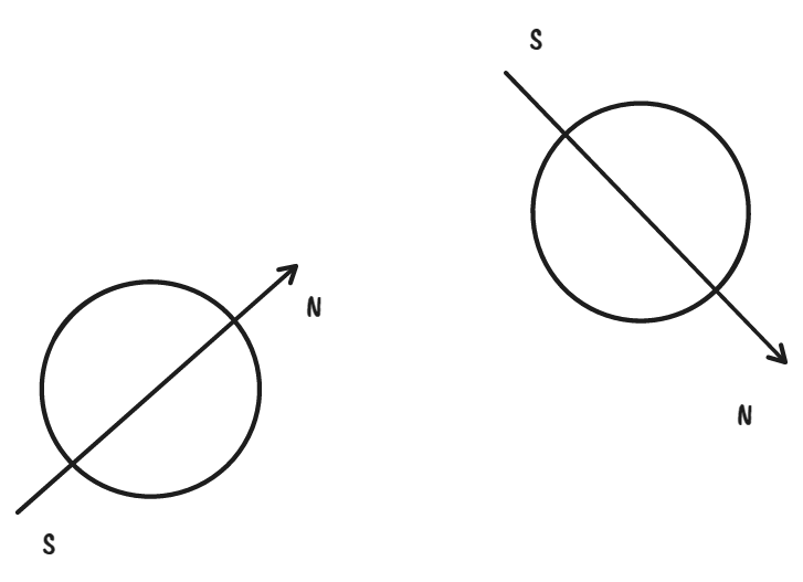
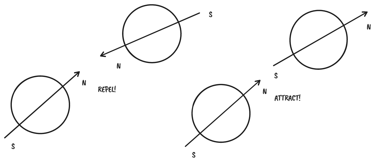
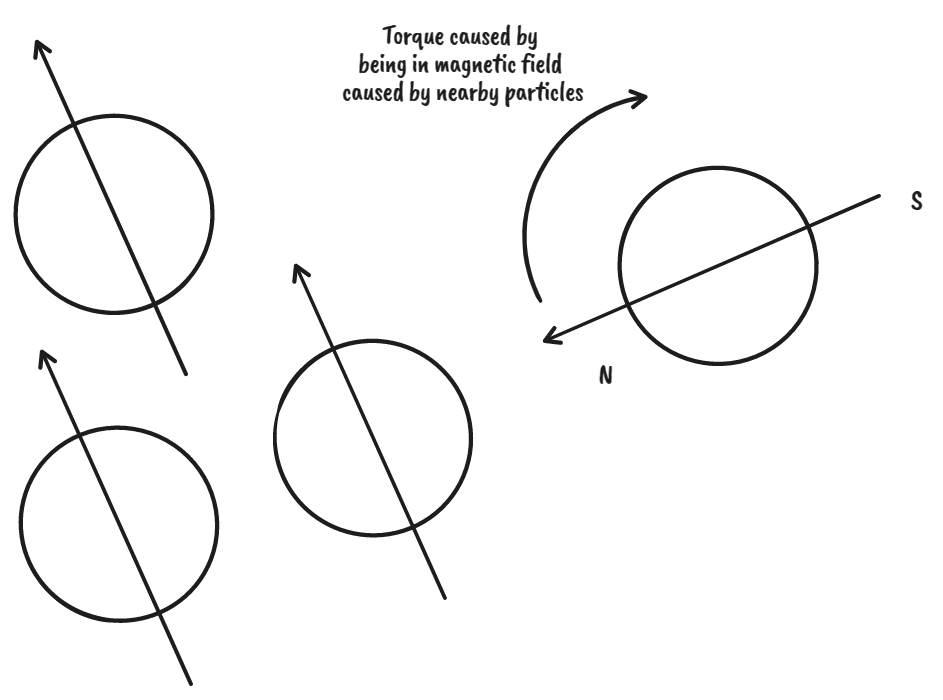
Dipoles are point-like magnets which have a positive and a negative pole both bunched up together infinitesimally close together. We could think of them as points that have an arrow vector attached, called the magnetic dipole moment. Dipoles attract each other just like bodies under gravity, however the forces are dependent on the alignment of the dipoles. As in any magnet, if the dipoles are aligned so they face each other with their north or south poles, they will repel. If they face each other with opposite poles they will attract. In between these alignments, the force will be dependent on their alignment via the vector dot product (more on this later…). Intuitively, we can expect the behaviours we’ll see should be more subjectively interesting than in the gravitational systems.
I chose to represent the moment as an angle. This angle is subject to the magnetic field caused by particles around it, and while the force moving particles around results in linear acceleration, the force that rotates the dipole moment is called torque and results in angular acceleration (aka change in rotation speed). These both have different equations that are a bit more complicated than for gravity.
To summarise these forces (or the accelerations they cause) though, they are:
The Linear Force F
The Torque T
You’ve made it this far and we’re talking about spicy things like magnetic dipoles, so we need to look at some equations. They are actually quite simple though, and this comes from the Wikipedia article on dipoles. I found that once I typed these into code, they were trivial and made me feel extremely clever having elucidated the mysteries of the magnetic vector field, which we call B.
r is the vector from the position of the dipole to the position where the field is being measured
r is the absolute value of r: the distance from the dipole
r̂ = r/r is the unit vector parallel to r;
m is the (vector) dipole moment
μ0 is the permeability of free space
Basically when we compute this, it gives us a vector pointing in the direction of the magnetic field at this point, and this vector will have a length indicating how strong the field is too. You might notice this weird “permeability” thing. This is a free parameter that is fun to play with and is basically just a magnetic equivalent of the G gravitational constant - it affects how strong our magnetic forces will be, globally.
Ok, we’ll come back to that in a moment. Here’s how to compute the linear acceleration. The force exerted by dipole M1 on M2 is:
where r is the distance between dipoles and m1, m2 are the moments of the two dipoles. The force acting on M1 is in the opposite direction. As you can see, it’s dependent on the alignment of the dipoles, as I said above, and we can guess this from seeing that a bunch of dot products between the moments are involved (dot products measure how aligned two vectors are). All we have to do is plug this into some code (it’s just a couple of lines especially if your language supports vector types and dot products), and we’re done.
So we know how to get B (the magnetic field at a point), and F the force by one dipole on another. B is used to calculate the torque, and this is actually quite simple.
The torque is simply the cross product between the moment of the dipole and the direction of the field at that point. The intuition here is that our magnetic moment is like a “lever arm”, and the magnetic field is like a force applied to that arm. When the dipole is perpendicular to the field, it will be rotated by the field until it becomes aligned.
Turning this torque into an angular acceleration is a bit tricky. Normally the formula to convert requires a Moment of Inertia of the object being rotated, but MOI for the dipoles would be mass times the distance to the axis of rotation squared… which would be 0. Oops. I wasn’t sure what to do about this so I pretended both of these are exactly 1 and just introduced a made up scaling factor for the torque’s strength, which can be user tweaked.
Basically all it means is that masses move toward each other using a law similar to gravity, but scaled by the dot product of moments, and they are rotated to conform with the magnetic field created by nearby dipoles. One interesting thing to notice is that the B field is more of an inverse cube, unlike gravity, as we are dividing by distance cubed.
So we simply accumulate the linear acceleration and torque on a particle by particle basis, just like we do for gravity, then once we’ve added up all these forces we add the total linear acceleration to the velocity and the total torque to the angle.
There are some useful details here.
It’s useful to add damping to both angular and linear velocity, otherwise both can be accelerated to huge speeds. The torque in particular can cause the angle of the particles to oscillate wildly, perhaps never quite aligning with the field since we are updating the simulation at discrete time steps. Basically all we have to do is multiply both velocities by a value between 0 and 1 at each update step, and this will make it as if they are experiencing drag in pool of liquid.
The distances involved (r) should be usefully scaled and clamped similar to the gravity scenario to avoid singularities and non-useful distance scales, I expose both a clamping range and a general distance scale in my program
OK one more thing. I also kept gravity around, except as a repulsive force. When particles are close together enough (i.e. I don’t activate this force above a certain distance at all, so it doesn’t accumulate at large scales), particles repel using the same gravity as in the previous section but with a negative sign. This keeps the particles from collapsing into tiny clumps or approaching singularity-like distances. The distance scale and strength of this force is also a free parameter that results in very different patterns.
Phew.
There is a problem though! The quadtree wasn’t designed to store dipoles. We have a centre of mass per box, but we don’t have a moment vector. We have to add together the moments from all the particles in a box too, to create an average moment, so we can pretend there are huge distant dipoles. This is where we have to take some liberties…
When we have a cloud of dipoles, the cloud itself becomes like a complex magnet with potentially many separated poles. I.e. it is no longer point like. I cheated here and pretended this is fine as an approximation though, so these distant quad tree cells simply have a huge powerful dipole at their centre of mass, with the moment given by adding together all the moments of the relevant particles.
So anyway, how does this look? What can we do with it?
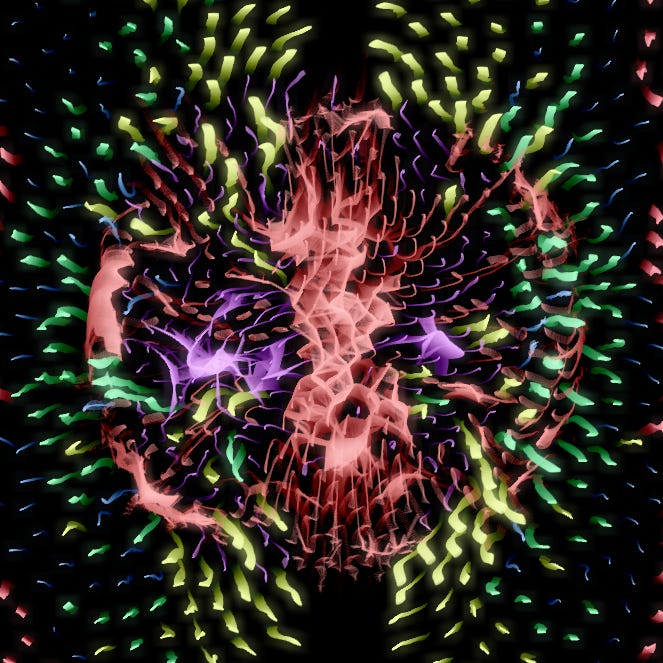
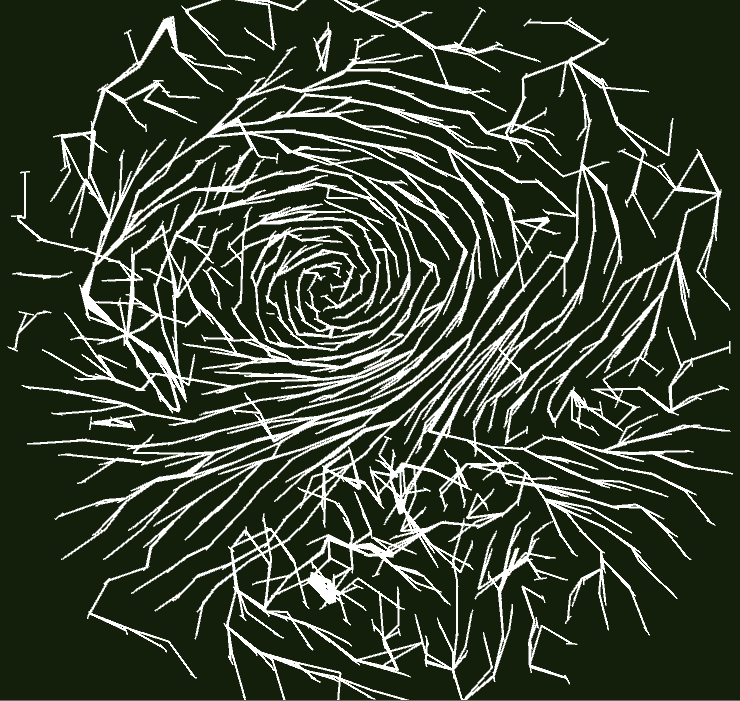
One thing that is interesting about this particle system is that rendering it as little dots doesn’t reveal the true self-organising structure. But if we draw them as tiny line segments representing the dipole moments, we will see some cool stuff. I also chose to scale the lines by the linear velocity of the particles, to give it some dynamism.
It looks… magnety. As you can see, the structures generated are related to the magnetic field lines generated by all of these interacting dipoles. It might remind one of the classic experiment of strewing lots of iron filings into a dish above a magnet, however iron filings aren’t (strongly) magnetic so they only rotate to follow the magnet’s field lines. Actually here’s a generation reminiscent of that:
In our case though, there is no single magnet - it appears as if these clouds of dipoles acts as one larger, continuously evolving magnetic field. Depending on starting conditions and random chance, multiple poles of different shapes can appear, swirl, move around and dissipate resulting in some interesting patterns. It is an n-body chaotic system, but governed by the rules of magnetism. Cool!
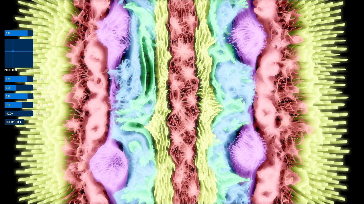
These are the free parameters I exposed to the user to play with:
d - the scaling of space for the magnetic field
u - the permeability
t - the torque strength
vd - the linear velocity damping
rd - the angular velocity damping
Perhaps the most important one of these is the spatial scaling. This controls on what scale the magnetic field lines end up occurring, so we can choose to have tiny ones or huge ones take take up the whole world - as if we had zoomed into a smaller system.
In the process of getting this all working, I also had some bugs (switched signs in various equations, for example), and I saw interesting emergent systems like these “cell walls”.
Magnetic Particle Life
After I’d had a bunch of fun playing with the parameters, I decided it’s cool but not as cool as it ought to be. I decided to add ideas inspired by Particle Life. Here’s how it works.
Instead of just a single type of particle, we create a family of them, each with different properties. Immediately this sounds exciting as it’s reminiscent of actual particle physics. The way this works is by creating an interaction matrix, that defines how particles affect each other - for example each matrix slot can say whether two particle types interact at all, how strong their magnetic pull is, how strong the repulsive force is (and perhaps it is attractive!), how strong the torque is, etc.
It is fairly simple to create RANDOM button that will just randomise all aspects of this matrix. Here are some cool results.
As you can see, it’s quite reminiscent of particle life but with the distinct visual hints of magnetic field lines. There are even these multi-cell floating objects that can move together. I’ve not finished exploring what's possible with this system yet (particle life is known to contain some very interesting pseudo-creatures, for example).
One thing I had to do here of course is separately store centres of mass and dipole moments per particle type per quadtree block, so that when the Barnes-Hut algorithm runs it can correctly add up the influences between the particles that can actually interact and given their specific rules.
However, at this point I hit a snag which I hope to rectify in a future article. The full Barnes-Hut magnetic simulation considering multiple particles types and running at scale is quite slow in my P5 project, meaning it doesn’t currently run at a solid framerate with the number of particles I want to render. This is even worse when doing the stuff I go over in the next section. Additionally, the artefacts caused by the approximation can be quite jarring if the approximation range is reduced enough to run well. This is partially because the monopole equations are much more computationally expensive than the simple repulsive/attractive force ones.
I’d like to try to re-create this system in a compute shader, but alas it would surely lose the immediacy of messing around with it in Processing. In the mean time, I have been able to at least render some videos offline with many particles.
Other Cool Stuff
When looking for some interesting ways to visualise the heavily directional vibes of the simulation, I tried one approach I quite liked.
This black metal album cover-looking image is drawn by linking particles with lines, in a way that follows the magnetic field lines. By using the quad-tree, we can query to find the nearest particle for any given particle. This can be used to draw a slightly cliché nearest-neighbour graph. But if instead of looking for the nearest particle we look for the nearest particle that is most aligned in terms of magnetic moment and also most “in the path” of the current one, we can connect them into longer curves this way. I also wrote some code so that these connections between particles linger statefully until particles stop matching for enough long enough, which really stabilises the links.
Here is the same algorithm in motion:
If we filter candidates based on alignment (using the dot product of their dipole moment vectors) and then sort by distance from the axis given by the particle and its moment, we can create these cool “preferential” tendrils that link particles along magnetic field lines.
Here’s another experiment combining the particle-life style rules with the connecting lines, but only partially clearing the background color between frames in P5, resulting in trails.
What About The Stanford Video?
While, I could never quite replicate the behaviour of the particles in the Stanford video, I was able to replicate some similar behaviours. Actually, if we add collision to the particles, we almost immediately start seeing particles form chains. It’s the formation of these chains that told me my implementation was on the right track as I’d seen them appear in various papers I was reading about ferro particle simulations.
So it’s not quite what was happening in the video. They were using electrodes and the type of fluid probably also matters. To simulate the concept of particles being “animated” by forming electrical connections, I tried to hack around with giving the particles a variable magnetisation, so they’d start non-magnetic and become magnetic by touching any particle that is in contact with an “electrode”, in my made up simplified fake physics. Here’s what it looked like.
It was ok but I didn’t follow up on this enough and my implementation of particles being linked this way was a bit buggy so I shelved it, at least for now.
Well, that’s it for now! Hope you enjoyed this article and learned some stuff or got some interesting ideas to experiment with.

